So, collecting Distributed Acoustic Sensing (DAS) data is the new and cool thing to do when it comes to seismic monitoring in oil and gas, mining and geothermal these days, but what actually is DAS measuring and how does this compare to traditional “point” measurements of ground motion made from geophones and seismometers? That is what we are going to address here, and along the way we’ll discuss some of the fundamentals of DAS measurements from a geophysical perspective. Then finally I’ll show how some common rules of DAS sensitivity (I call them DAS’isms) can be obtained from a very simple and much more general starting point. I do this for several reasons:
- To explain why DAS data should be treated differently from standard seismic data.
- To describe where the “rules” for DAS sensitivity (such as cosine-squared sensitivity) actually come from so that we know what they approximate and what the do not.
- To correct some mis-conceptions that might still be out there.
- To provide a basis I can refer back in order to start doing some really fun stuff.
Who is this all for? I hear you ask. Well if you are a geophysicist or seismologist who wants to understand a bit more about DAS data particularly from a theoretical standpoint then this page is for you. There is a little bit of math but I have tried to set things out in such a way that if math is not your thing then you can just gloss over it a read the text. Those who are already very knowledgeable on DAS systems I expect won’t find anything too surprising here. However, the line I am going to take is a little different compared to what most talks and papers take, so you might still gain some benefit from seeing familiar material described in a different way.
What Does DAS Measure?
In my opinion the term DAS is somewhat misleading name for seismic measurement from a fibre optic cable. DAS stands for Distributed Acoustic Sensing, the “Distributed” bit is quite accurate (as we will see) and the “Sensing” bit I don’t have a problem with either, it is the “Acoustic” bit I have difficulty with. This is because, as a geophysicist, when I hear the term Acoustic I think of sound/ pressure waves in gas or fluid described by a scalar wave equation but this is not what DAS is measuring. When DAS is employed as a seismic sensor you are measuring strain in the fibre optic cable. It has been pointed out to me that more general physicists used the term acoustic to describe the propagation of vibrations in solids so the term is not strictly wrong. plus everyone is already calling it DAS so this is the term we will use as well. However, it is important to remember as we go that DAS applied as a seismic setting is a strain sensor.
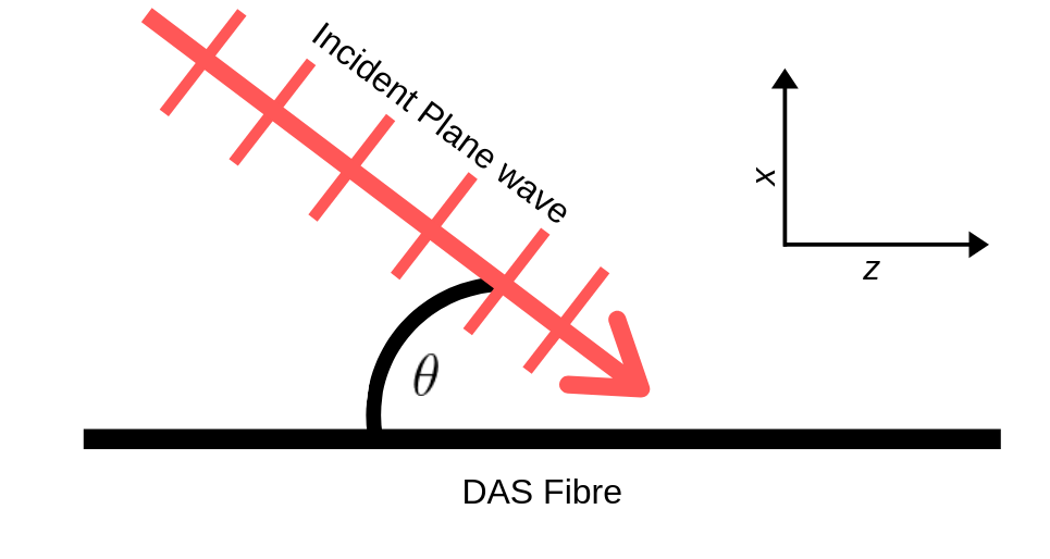
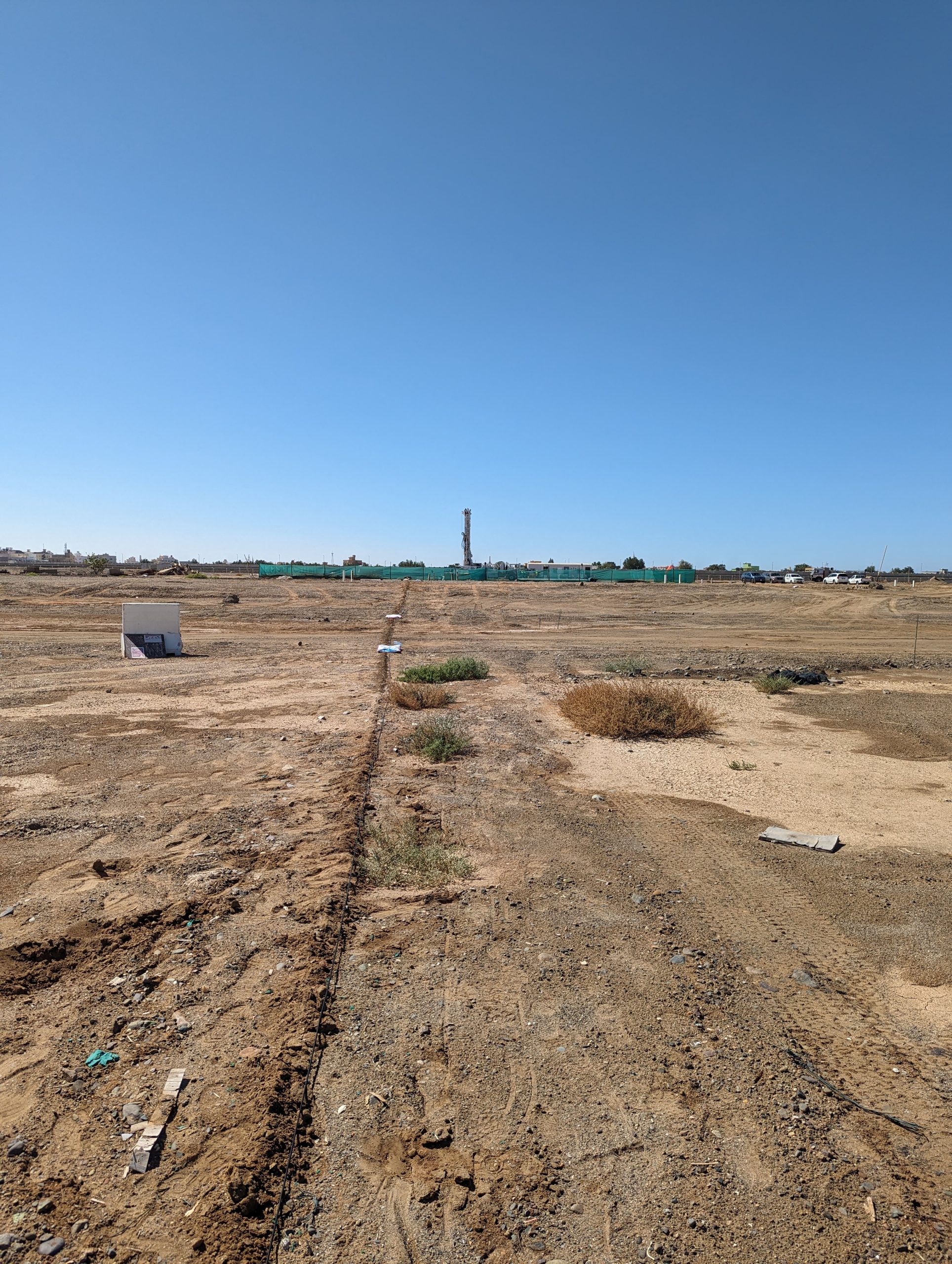
So how does the measurement work? This is a massive topic in itself which a lot of very clever people have worked very hard on. Needless to say there are all sort of specifics which vary with the different systems and deployment scenarios (downhole, surface trenched, behind casing …), but for our purposes here a simple drawing will suffice.
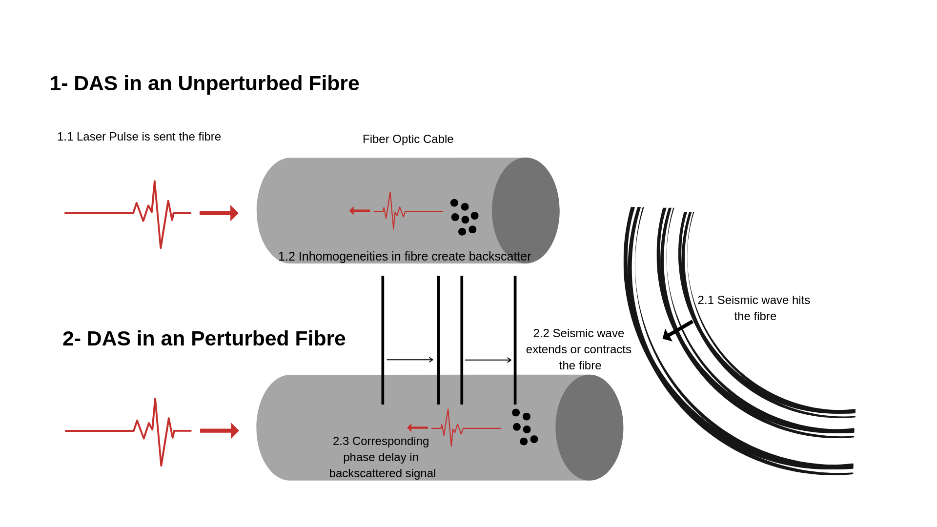
Essentially a laser pulse is transmitted down the fibre optic cable, which is backscattered by inhomogeneities in the fibre. Then when the fibre length changes due to an incident seismic wave (or some other effect) it produces a corresponding phase delay in the backscattered pulse which can be detected. The concept is in fact somewhat similar to that used in Interferometric Synthetic Aperture Radar (InSAR), where phase difference between two pulses reflected off the Earths surface is used to measure ground deformation from satellites.
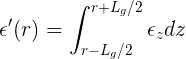
So taking the above drawing at face value what DAS is actually measuring is length change in a fibre optic cable. However, in practice DAS systems typically convert this phase difference into a relative length change (i.e. strain) over a finite distance called the gauge length. This is because the incident laser pulse has a certain length and by averaging over a longer piece of fibre the amount of backscattered energy is increased. Following Harthog (2018) p348 the “effective” strain measured by the DAS system is given by
where
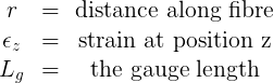
Note that this formula is just a fancy way of saying DAS output at point is the average of the strain at all points in the fibre either side of that point up to half the gauge length. I would also add that many systems measure strain rate, rather than direct strain as show above but this does not really effect the points made in the rest of this article other than to introduce a time derivative (i.e. convert displacement to velocity).
How do DAS measurements relate to standard seismic data?
Standard seismic data is the name I am going to use for data collected with either seismometers or geophones. Again there are a ton of specific details associated with both of these instruments, but for our purposes it is enough to say they both effectively provide point measurements of ground velocity. This is important to remember because most of the techniques we use for quantitatively analysing seismic data are based on the measurement being taken at a point. Something which is not the case for DAS.
Strain is the related to displacement, and similarly strain-rate is related to velocity by a spatial gradient. Mathematically this is written as
![]()
where
![]()
In other words the strain or strain-rate as measured by DAS is related to the spatial gradient of displacement or velocity as measured by a standard seismic instrument. Those who are particularly astute will note that I am just using 1 component of the strain tensor in order to keep things simple here, but the argument holds in a general sense provided you rotate the strain tensor to be aligned with the fibre direction.
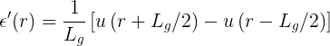
Putting this together with the averaging equation from the previous section you get a general equation for DAS strain or strain rate a function of displacement or velocity at either end of the gauge length
 So that’s really nice but what does this mean?
- The above equation tells us that the strain or strain-rate as measured by DAS is effectively the difference between 2 displacement or velocity sensors placed at either end of the gauge divided by the gauge length.
- And taking that further it provides a way to “simulate” a DAS recording, all you have to do is place standard seismic sensors at either end of your gauge and difference them.
- It also tells us that although in DAS surveys we might be collecting data based on the central position in the gauge, it is actually what is happening at the ends of the gauge that really determines the output signal.
- Finally, it provides a basis for explaining rules of thumb for DAS sensitivity with incidence angle.
The relationship is fairly general, for example, it does not make any assumptions about the incident energy (P-wave, S-wave, etc.). The formulation does assume that the fibre is straight over the gauge length, but with a minor modification it can be adapted to non-straight fibre’s. In short it provides a good basis from which to study more specific cases.
Can you Convert DAS Data Into Point Sensor Data?
In principle, yes, and this has been done by several people for purposes of comparing DAS and geophone/ seismometer datasets (for example see the link to Mark Willis’s EAGE lecture below). However what the above formula tells us is that you cannot do so without making some assumptions.
Those who are knowledgable on such things might recognise that determining the geophone response at the gauge ends as a linear inverse problem and we could write it in a matrix form which would look something like this
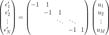
Where the left hand side are the DAS measurements, and the vector on the right are point displacement or velocities we want to determine at the end of the gauges. They are related by a differencing matrix. The problem is that in order to solve for the right hand vector it is necessary to invert an inner product matrix derived from that differencing matrix, which will be rank deficient (i.e it will always have at least one eigenvalue which is zero). This means that the model space has more degrees of freedom than the data space, or that there are signals which could be present in the velocity or displacement data which cannot be seen in the DAS data. A simple example of this is a DC shift (i.e. constant velocity or displacement) could in principle be recorded by a point sensor (albeit not with standard equipment), but cannot be seen in the DAS signal.
For the most part though, the signals which cannot be represented in the DAS data are not the ones we are after in geophysics and there are techniques for handling ill-posed inverse problems such as the one above (e.g. SVD or adding a linear constraint). So we can re-construct a point sensor responses from DAS recordings, however, it worth keeping in mind that this approach is mathematically incomplete. Arguably a better approach for comparing DAS and geophone or seismometer data is to run the problem forwards and use the velocity or displacement records to simulate a DAS response.
Deriving DAS Responses
We’ll now put the analysis above to good use in order to provide DAS responses for incident P and S-waves. In the process we’ll verify two DAS’isms namely:
- The P-wave response of the fibres depends on the squared-cosine of the incidence angle.
- The S-wave response depends on the sine of twice the angle of incidence.
The incidence angle is the angle between the the waveform normal and the fibre,
As we’ll see these DAS’isms are in fact approximations of a more general response for a DAS fibre which depends on both the incident frequency as well as the incident angle.
Incident P-wave
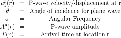
Using the above derivations and a formula for a planar incident P-wave displacement
![]() where
where
you can obtain an expression for the effective strain recorded on the DAS which looks like this
![]()
Written this way the term in the brackets can be thought of as a spatial and frequency filter associated with a DAS response compared to the geophone response (which is just the cosine times amplitude). Or in other words if you have a point measurement of an incident plane wave you get the first two terms (cosine of the incidence angle times the amplitude), but if you have a DAS system the subsequent terms act as a spatial frequency filter to distort this signal. Exactly how the signal is distorted depends upon the incidence angle and the frequency content. We can now compute an amplitude response spectrum for a DAS system to a plane wave as a function of frequency and incidence angle to get
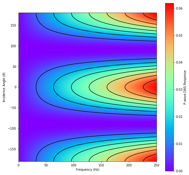
To make the above plot I assumed gauge length (L) of 10m and P-wave velocity of 2500 m/s. From the figure we can see that as the incidence angle tends to 90 degrees (i.e. the incident wave hits the fibre at right angles) the fibre response tends to zero. Similarly the highest responses are seen where the incident wave is travelling parallel to the fibre (zero and 180 degrees incidence). There is also a frequency/ wave number effect where by lower frequencies are attenuated due to there being less difference in the signals between the ends of the gauge. Finally, if we took a cross-section though the above plot at constant frequency we would obtain a function proportional to cosine of the incidence angle squared and obtain the the first DAS’ism.
Incident S-wave
We can do the same thing for an incident S-wave, however, we have to consider the incident S-wave velocity/displacement as a vector projected into the direction of the fibre to obtain
![]() Applying the same substitutions as with the P-wave we get a similar expression to what we had for the P-wave
Applying the same substitutions as with the P-wave we get a similar expression to what we had for the P-wave ![]()
In fact, the DAS response filter (the term in brackets) is the same as before, which makes sense since the fibre geometry has not changed. It is just the initial terms describing the incident S-wave which are different. Computing the amplitude response as a function of frequency and incident cosine (relative to the fibre) we get the following spectrum
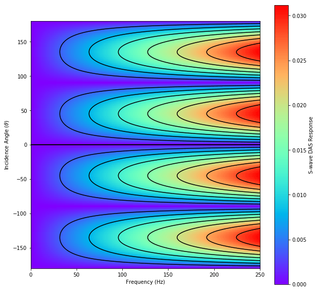
As before I assumed gauge length of 10m, but have replaced the velocity term with a more realistic S-wave value of 1560m/s. Unlike the P-wave we get nulls in the S-wave response for incidence angles parallel to the fibre because in this case there will be no particle motion in the fibre direction. Similarly there are nulls in the DAS response when incidence is perpendicular (incidence of 90 degrees) as in this case there is no relative motion between the gauge ends. Finally considering a cross-section through the above plot at constant frequency the second DAS’ism is obtained, namely that the S-wave response of the fibre with incidence angle follows a sin2θ pattern. However, because the plot shows an amplitude response spectrum the polarity reversal is not seen, but this is captured in the corresponding phase spectrum.
Summary
If you have stuck with me this far then well done, and hopefully you have gained some insights along the way into how DAS operates and how these measurements compare to standard seismic data measured by geophones or seismometers.
Now for those who just skipped to the end, the keys points are as follows:
- DAS is not strictly and acoustic measurement, it is a strain measurement.
- DAS recordings are related to the difference in displacement or velocity measurements at either end of the gauge length.
- Once we understand point 2 the some other DAS’isms such as DAS fibre’s sensitivity with incidence angle follows a cosine squared for P and sin2θ for S become apparent.
Hopefully this has left you a bit more knowledgable regards how some the properties of DAS measurements interact. As always feel free to get in touch if you would like to discuss this in any more detail.
Acknowledgements References and Useful Links
Let me start by thanking an anonymous DAS industry professional for their input on an original draft of this page. Now there are bewildering number of papers and conference abstracts on this topic. Rather than try to list them all I thought I would provide 3 examples that give a good general background and are not directly associated with a vendor or product. Nonetheless MST is providing these resources on an entirely use at own risk basis, without any acceptance of warranty or liability…. you get the idea. Similarly the authors and publishers have not been consulted regards placing links to their work here, nor are they considered to be affiliated or endorsing MST in anyway. In short the links are here because I hope people will find them useful and the authors/ publishers want their work linked too.
- Harthog, An introduction to distributed optical fibre sensors, CRC Press (2018) – Provides a very comprehensive (some would say exhaustive) overview of the applications and ways in which DAS systems work.
- https://www.youtube.com/watch?v=gs3SQoe5w8Q – A 15 minute YouTube video from EAGE featuring Mark Willis discussing comparisons of DAS sensors with other measurements.
- https://www.youtube.com/watch?v=LAcQ44YRMuM– A 30 minute YouTube video explaining some of basic ideas behind DAS given by Nate Lindsey (Berkley) and Eileen Martin (Virginia Tech).


