One of my side-projects is examining a dataset collected at the Brady Hot Springs geothermal field in Nevada, where in March 2016 an extensive and multi-faceted survey was undertaken (called the PoroTomo project). The project resulted in many published papers and conference proceedings (see reference list for details), but my interest in this dataset stems from two factors:
- I believe that although a lot of good work has been done on the data collected, but like many large geophysical projects, there is still a lot this data has to tell us. Much of the geophysical work presented on this data so far has focussed on the detection of seismic activity and delineation of geothermal reservoir properties. However, I think this dataset can also be used to demonstrate the monitoring of transport and infrastructure using DAS fibres.
- The data is free and publically available from the Geothermal Resources Council and the University of Wisconsin (see the section at the end for links). By making the data publically available the project leaders have created an excellent resource for small companies and research institutions to innovate and present new ideas. Personally, I cannot put into words just how grateful I am that they have done this.
With that in mind, I should add that MST was not in any way involved with the PoroTomo project or the collection of this data. At the time of writing, the only information I have about the project is what is publically available. That said if anyone involved with the project is reading this feel free to get in touch, and I would be happy to share more details about the analysis with you. What follows should not be taken as an endorsement for any external vendor/ institution or service. All the processing was performed using MST’s proprietary processing platform (MSF-lab).
The Surface DAS Deployment
Two DAS systems were deployed at the Brady Hot Springs site, a system in a vertical wellbore and cable deployed horizontally near the surface. In what follows we’ll be dealing with the near-surface horizontal deployment. The following figure shows a map view of the sensor layout with every 1000’th sensor labeled.

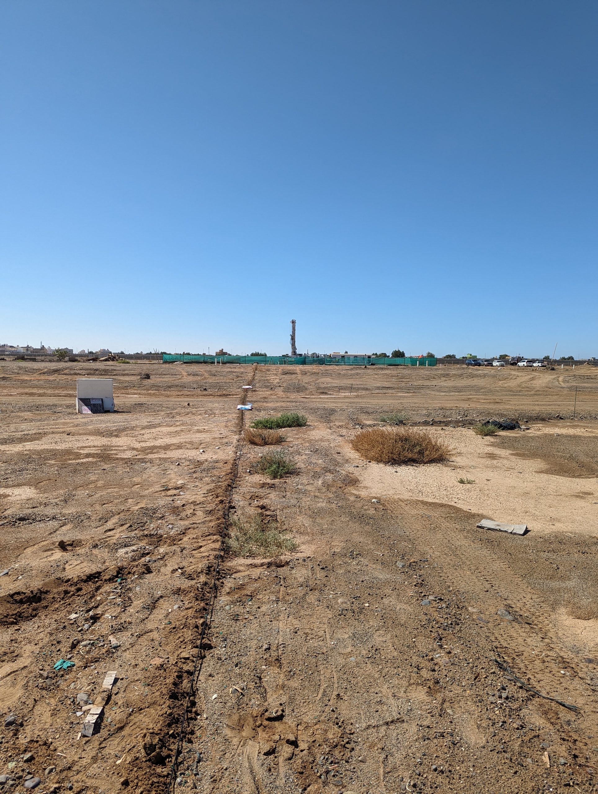
The total fibre length is about 8.7km, with overlapping sensing segments of 10m length (i.e. 10m gauge length) spaced at 1m intervals. In practice, there are some auxiliary channels at the start and end of the fibre making a total of 8621 sensors. The cable was deployed in a shallow trench, and data was collected over about 15 days. As can be seen from the figure, in addition to activity associated with the geothermal system there are a number of other potential sources of interesting signals in the data. For example, there is a major highway running right along one side of the array as well as smaller roads and buildings.
Getting the Data
As mentioned above the recorded data is freely available from the University of Wisconsin FTP and GRC resource website. However, the dataset is relatively large (approx 30TB and distributed over about 40,000 SEGY files), so the first task is to organize the data such that we can select the bits we want in a scalable fashion. To this end, I created a cloud storage area containing compressed versions of the data files. The data compression resulted in an ~97% reduction in data volume, thus minimising cloud storage costs and increasing retrieval speed (i.e. reduced network traffic). Once in place, the data was indexed such that we can rapidly select the segments we need for analysis.
Initial Results
One of the first things we can do with the DAS data is to construct waterfall plots. If you have worked with DAS data before you’ll probably be familiar with waterfall plots, if you have not, they are just plots showing some time window summary of the data vs channel number. For example, the following waterfall plot shows RMS calculated over 15 second windows for 2 days of data from the array.

In the plot, Y-axis shows channel number (see map for the channel locations) and X-axis time, each pixel is the RMS computed in that 15 second window. The white panels are time intervals with missing data, whilst the horizontal red line corresponding to channel ~4750 matches up with a location of a dry river bed. Presumably, the cable is deployed differently at this location, for example, perhaps it is not trenched as deeply resulting in high noise channels. A particularly striking feature is the high levels of an activity forming an X during the day on the 13th of March. These high amplitudes are almost certainly related to the vibroseis crew that was shooting seismic at the time (also as part of the PoroTomo project). Note that the X pattern is created by a combination of the movement of vibroseis crew from NE to SW during the day combined with the sensing cable curving back on itself. Unfortunately, the interference from the vibroseis makes looking for other activity during these time periods challenging.
Traffic On the Highway
Fortunately, there are several extended periods when no seismic was being shot. For example, the following figure shows the same data but for 12 hours overnight.

One particularly noteworthy feature is the vertical banding on the first 4000 sensors. Recall that these sensors are the closest to the high way, so it seems likely these are the signals from passing vehicles (probably trucks) on the highway. The examination of shorter time segments confirms this

In the above plots, the black vertical line on the left-hand waterfall plots shows time-slice plotted on the array on the RHS. Notably, from the waterfall plot, we can see the signals from several vehicles moving along the highway. The majority seem to be traveling NE to SW (the signals are visible earlier on sensors in the NE of the array). This probably reflects an asymmetry in traffic movements, since we would expect traffic moving SW to NE to be more readily detected by the array since it will be on the side of the road that is closer to the sensors. The approximate time delay of signals moving across the array (about 60 seconds) is consistent with velocities of roughly 25m/s or about 60 miles per hour. However, this is only a rough estimate because the zig-zag pattern of the cable also creates apparent time delays.
Some sections of the cable also show much larger signals from the cars compared to others. This could be due to site or path effects, for example in some areas the cable may be more sensitive due to better coupling. However, as explained in one of my other articles (What Is DAS And What Is It Measuring?), since DAS is a finite strain measurement there is also a directional sensitivity of the fibre. So, since the fibre zig-zags back and forth we might expect different sections of the cable to record different responses for the incident energy.
What now?
The deployment at Brady Hot Springs is clearly a somewhat unusual case (although there are other Geothermal sites where DAS is being used in DH configurations) to use DAS for monitoring traffic patterns given its remote location. However, DAS systems are deployable in a number of other environments for transport and infrastructure monitoring. As such, I believe this dataset can be used to demonstrate some of the many applications for DAS in addition to monitoring the geothermal reservoirs. For example:
- Can we apply more sophisticated processing algorithms to extract more subtle signals from the data?
- Can we examine the traffic patterns on the high way in more detail?
- Can we detect accidents or stopped vehicles or vehicles behaving erratically (for example if the driver is under the influence of alcohol or drugs)?
- Can we use the signals from traffic to monitor the condition of the highway?
As indicated by the “Part 1” in the title of this post, I intend to come back to some of these things in future posts. Stay tuned for updates.
Data
Links to the DAS data for the project at Brady Hot Springs as well as other metadata are available from the Geothermal Data Repository.
References
The following are just some of the papers and conference proceedings published on the Brady Hot Springs data. If you have or know of, a publication you would like me to add feel free to get in touch
Feigl et. al. (2017), Overview and preliminary results from the3 PoroTomo project at Brady Hot Springs Nevada: Poroelastic tomography by adjoint inverse modeling for data from seismology geodesy and hydrology, Proc. 42nd Workshop on geothermal reservoir engineering. Stanford, California.
Li and Zhan (2018), Pushing the limit of earthquake detection with distributed acoustic sensing and template matching: a case study at the Brady geothermal field, Geophys. J. Int., 215, 1583-1593.
Matzel et al. (2017), Using virtual earthquakes to characterize material properties of the Brady Hot Springs, Nevada, GRC Transactions, Vol 41.
Miller et. al. (2018), DAS and DTS at Brady Hot Springs: Observations about coupling and coupled interpretations. Proc. 43rd Workshop on geothermal reservoir engineering. Stanford, California.


